Contents
How to use GBQ
Note that the data should be located in Google cloud, whether in Google Cloud Storage, Google Drive, Cloud BigTable, or output from any Google’s SaaS.
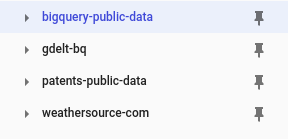
Google BigQuery also provides a number of public datasets that make users easier to combine instantly with their own dataset such as NOAA, Bitcoin, WorldBank, census, flights, taxi, GitHub, Wikipedia, etc.
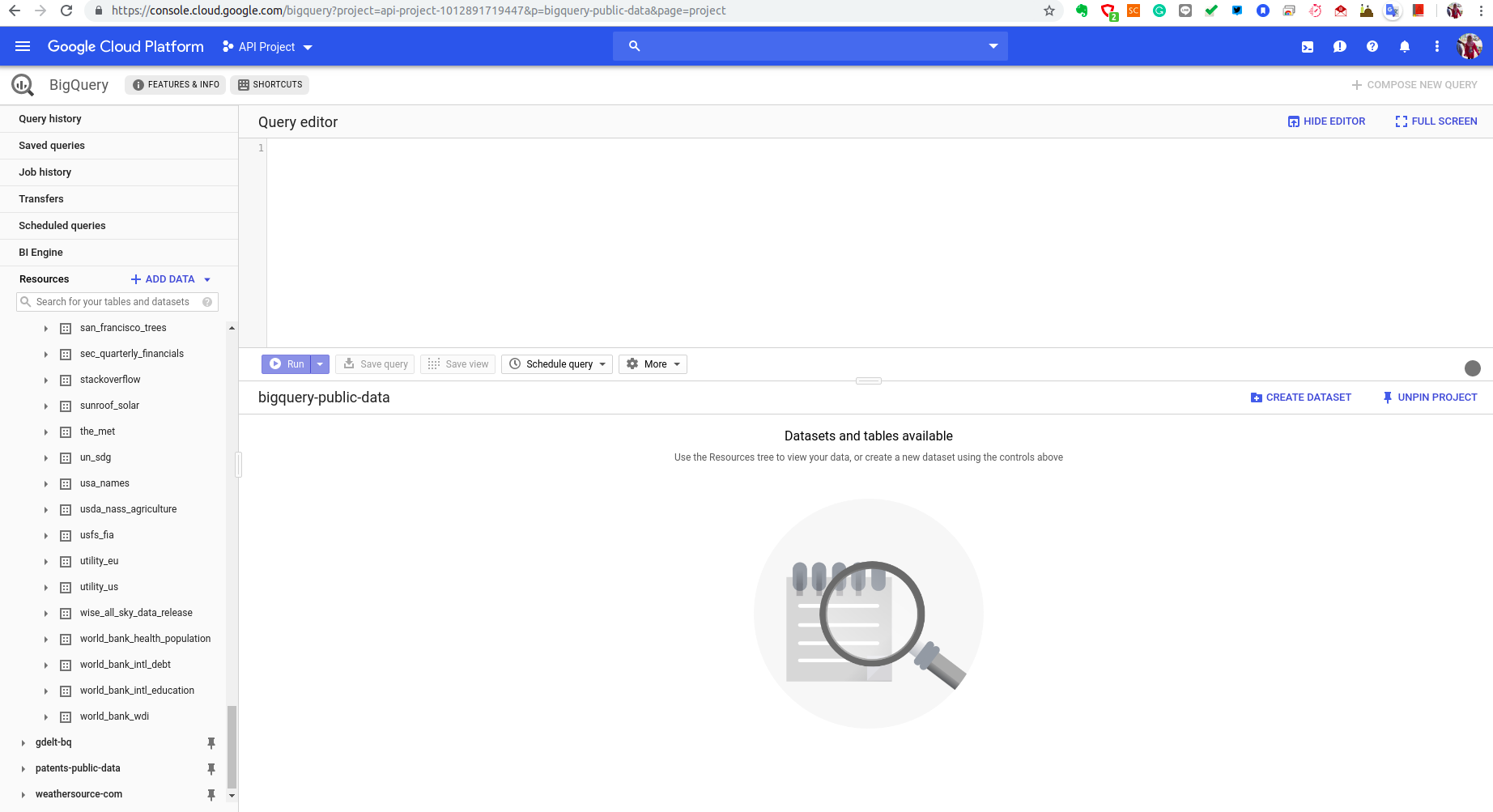
There are many ways to use Google BigQuery such as via GCP’s user interface, console, SDK, REST API, etc. The easiest way is using the UI, but for the sake of reproducibility, we use SDK in this article. Installing Google Cloud SDK is very straightforward. The official guide from Google provides clear instruction on how to do that.
Basic Operation
No | Objective | CLI command (example): | Python client (example): |
|---|---|---|---|
| Installation | wget https://dl.google.com/dl/cloudsdk/channels/rapid/downloads/google-cloud-sdk-249.0.0-linux-x86_64.tar.gz tar -xvzf google-cloud-sdk-249.0.0-linux-x86_64.tar.gz cd google-cloud-sdk && ./install.sh | conda install -c conda-forge google-cloud-bigquery (or pip install --upgrade google-cloud-bigquery --user) | |
| Initialization | gcloud init \ --console-only \ --skip-diagnostics | from google.cloud import bigquery client = bigquery.Client(location="US") | |
| Listing all datasets in a project (option 1) | bq ls \ --max_results 50 \ --format prettyjson \ --project_id myproject | datasets = list(client.list_datasets("myproject")) for dataset in datasets: dataset._properties | |
| Getting all datasets in a project (option 2) | bq query \ --nouse_legacy_sql \ --project_id myproject \ 'SELECT * EXCEPT(schema_owner) FROM INFORMATION_SCHEMA.SCHEMATA' | job_config = bigquery.QueryJobConfig() sql = 'SELECT * EXCEPT(schema_owner) FROM INFORMATION_SCHEMA.SCHEMATA' query_job = client.query(sql, location="US", job_config=job_config) for row in query_job.result(): print(format(row)) | |
| 1 | Create a dataset | bq mk \ --data_location US \ --dataset \ --default_table_expiration 3600 \ --time_partitioning_expiration 3600 \ --description "This is dataset about me" \ myproject:mydataset | dataset = bigquery.Dataset("myproject.mydataset2") dataset.location = "US" dataset.default_table_expiration_ms = 3600000 dataset.description = "This is dataset about me" dataset = client.create_dataset(dataset) |
| 2 | Getting dataset information | bq show \ --format prettyjson \ myproject:mydataset | dataset = client.get_dataset("myproject.mydataset2") dataset._properties |
| Getting all tables in the dataset | bq query \ --nouse_legacy_sql \ 'SELECT * EXCEPT(is_typed) FROM mydataset.INFORMATION_SCHEMA.TABLES' | dataset = client.get_dataset("myproject.mydataset2") tables = dataset.tables() for table in tables: table._properties | |
| 3 | Getting all table options in the dataset | bq query \ --nouse_legacy_sql \ 'SELECT * FROM mydataset.INFORMATION_SCHEMA.TABLE_OPTIONS' | job_config = bigquery.QueryJobConfig() sql = 'SELECT * FROM mydataset2.INFORMATION_SCHEMA.TABLE_OPTIONS' query_job = client.query(sql, location="US", job_config=job_config) for row in query_job.result(): print(format(row)) |
| 4 | Getting all columns of all tables in the dataset | bq query \ --nouse_legacy_sql \ 'SELECT * FROM mydataset.INFORMATION_SCHEMA.COLUMNS' | job_config = bigquery.QueryJobConfig() sql = 'SELECT * FROM mydataset.INFORMATION_SCHEMA.COLUMNS' query_job = client.query(sql, location="US", job_config=job_config) for row in query_job.result(): print(format(row)) |
| Getting column's structure from all columns of all tables in the dataset | bq query \ --nouse_legacy_sql \ 'SELECT * FROM `bigquery-public-data`.github_repos.INFORMATION_SCHEMA.COLUMN_FIELD_PATHS' | job_config = bigquery.QueryJobConfig() sql = 'SELECT * FROM `bigquery-public-data`.github_repos.INFORMATION_SCHEMA.COLUMN_FIELD_PATHS' query_job = client.query(sql, location="US", job_config=job_config) for row in query_job.result(): print(format(row)) | |
| 5 | Create an empty table in a dataset | bq mk \ --table \ --expiration 3600 \ --description "This is an empty table" \ --label department:marketing \ --label classification:important \ myproject:mydataset.mytable \ field1:string,field2:integer,field3:float | schema = [bigquery.SchemaField("field1", "STRING", mode="REQUIRED"), bigquery.SchemaField("field2", "INTEGER", mode="REQUIRED"), bigquery.SchemaField("field3", "FLOAT", mode="REQUIRED"),] table = bigquery.Table("myproject.mydataset2.mytable", schema=schema) table.description = "This is an empty table" table.labels = {"department":"marketing", "classification":"important"} table = client.create_table(table) |
| 6 | Creating a table from a query result | bq query \ --destination_table \ myproject:mydataset.mytable2 \ --nouse_legacy_sql \ 'SELECT * FROM `bigquery-public-data.ml_datasets.iris`' | job_config = bigquery.QueryJobConfig() table_ref = client.dataset("myproject.mydataset").table('mytable2') job_config.destination = table_ref sql = """SELECT * FROM `bigquery-public-data.ml_datasets.iris`""" query_job = client.query(sql, location="US", job_config=job_config) query_job.result() |
| 7 | Creating a table that references an external GCS | bq mk \ --external_table_definition=x:string,y:float@CSV=gs://agungw132-public/d.csv.gz \ myproject:mydataset.mytable3 | schema = [bigquery.SchemaField('x', 'STRING'), bigquery.SchemaField('y', 'INTEGER')] table_ref = client.dataset("mydataset2").table('mytable3') table = bigquery.Table(table_ref, schema=schema) external_config = bigquery.ExternalConfig('CSV') external_config.source_uris = ['gs://agungw132-public/d.csv.gz',] external_config.options.skip_leading_rows = 0 table.external_data_configuration = external_config table = client.create_table(table) |
| 8 | Creating a table that references an external GDrive | bq mk \ --external_table_definition=x:string,y:float@CSV=https://drive.google.com/open?id=183M8Am20cNutbs9UKKPL0R4dQyWPKb2L \ myproject:mydataset.mytable4 | schema = [bigquery.SchemaField('x', 'STRING'), bigquery.SchemaField('y', 'INTEGER')] table_ref = client.dataset("mydataset2").table('mytable4') table = bigquery.Table(table_ref, schema=schema) external_config = bigquery.ExternalConfig('CSV') external_config.source_uris = ['https://drive.google.com/open?id=183M8Am20cNutbs9UKKPL0R4dQyWPKb2L',] external_config.options.skip_leading_rows = 0 table.external_data_configuration = external_config table = client.create_table(table) |
| 9 | Creating a table in GCS from a query result (query success, but no file in bucket) | bq query \ --external_table_definition=mytable5::sepal_length:FLOAT,sepal_width:FLOAT,petal_length:FLOAT,petal_width:FLOAT,species:STRING\ @CSV=gs://agungw132-public-us/mytable5.csv \ --nouse_legacy_sql \ 'SELECT * FROM `bigquery-public-data.ml_datasets.iris`' | external_config = bigquery.ExternalConfig('CSV') external_config.source_uris = ['gs://agungw132-public/mytable5.csv',] external_config.schema = [bigquery.SchemaField('sepal_length', 'FLOAT'), bigquery.SchemaField('sepal_width', 'FLOAT'), bigquery.SchemaField('petal_length', 'FLOAT'), bigquery.SchemaField('petal_width', 'FLOAT'), bigquery.SchemaField('species', 'STRING'),] external_config.options.skip_leading_rows = 0 job_config = bigquery.QueryJobConfig() job_config.table_definitions = {"mytable5": external_config} sql = 'SELECT * FROM `bigquery-public-data.ml_datasets.iris`' query_job = client.query(sql, location="US", job_config=job_config) query_job.result() |
| Getting table information (metadata) | bq show \ --schema \ --format prettyjson \ myproject:mydataset.mytable | table = client.get_table("myproject.mydataset2.mytable") table._properties | |
| Getting table options of a table | bq query \ --nouse_legacy_sql \ 'SELECT * FROM mydataset.INFORMATION_SCHEMA.TABLE_OPTIONS WHERE table_name="mytable"' | job_config = bigquery.QueryJobConfig() sql = 'SELECT * FROM mydataset2.INFORMATION_SCHEMA.TABLE_OPTIONS WHERE table_name="mytable"' query_job = client.query(sql, location="US", job_config=job_config) for row in query_job.result(): print(format(row)) | |
| Getting all columns in a table | bq query \ --nouse_legacy_sql \ 'SELECT * FROM mydataset.INFORMATION_SCHEMA.COLUMNS WHERE table_name="mytable"' | job_config = bigquery.QueryJobConfig() sql = 'SELECT * FROM mydataset2.INFORMATION_SCHEMA.COLUMNS WHERE table_name="mytable"' query_job = client.query(sql, location="US", job_config=job_config) for row in query_job.result(): print(format(row)) | |
| Getting column's structure from all columns in a table | bq query \ --nouse_legacy_sql \ 'SELECT * FROM mydataset.INFORMATION_SCHEMA.COLUMN_FIELD_PATHS WHERE table_name="mytable"' | job_config = bigquery.QueryJobConfig() sql = 'SELECT * FROM mydataset2.INFORMATION_SCHEMA.COLUMN_FIELD_PATHS WHERE table_name="mytable"' query_job = client.query(sql, location="US", job_config=job_config) for row in query_job.result(): print(format(row)) | |
| 1 | Getting n first rows of a table | bq head \ --n 10 \ --start_row 1 \ --selected_fields "" \ myproject:mydataset.mytable | NA |
| 2 | Updating table properties (description, expiration_time, schema definition, labels) | bq update \ --description "This is updated description" \ myproject,mydataset.mytable | table_ref = client.dataset('mydataset2').table('mytable') table = client.get_table(table_ref) assert table.description == "Original description." table.description = "Updated description." table = client.update_table(table, ["description"]) # API request assert table.description == "Updated description." |
| 3 | Duplicating a table | bq cp \ --append_table \ --force \ --no_clobber \ myproject.mydataset.mytable myproject.mydataset.mytable_copy | source_table_ref = client.dataset('mydataset2').table('mytable') dest_table_ref = client.dataset('mydataset2').table('mytable_copy') job = client.copy_table( source_table_ref, dest_table_ref, # Location must match that of the source and destination tables. location="US",) job.result() |
| 4 | Copying multiple tables to a table | bq cp \ --append_table \ --force \ --no_clobber \ myproject.mydataset.mytable,myproject.mydataset.mytable2 \ myproject.mydataset.mytable_copy | source_table_ref1 = client.dataset('mydataset2').table('mytable') source_table_ref2 = client.dataset('mydataset2').table('mytable2') dest_table_ref = client.dataset('mydataset2').table('mytable_copy') job = client.copy_table( [source_table_ref1,source_table_ref2], dest_table_ref, # Location must match that of the source and destination tables. location="US",) job.result() |
| 5 | Deleting a table | bq rm \ --table \ --force \ myproject.mydataset.mytable | table_ref = client.dataset('mydataset2').table('mytable') client.delete_table(table_ref, not_found_ok=True) |
| 6 | Restoring a deleted table | bq cp \ mydataset.mytable@1559816526000 \ mydataset.newtable | import time snapshot_table_id = "{}@{}".format("mytable", int(time.time()*1000-200)) #200 second ago snapshot_table_ref = client.dataset('mydataset2').table(snapshot_table_id) recovered_table_ref = client.dataset('mydataset2').table("newtable2") job = client.copy_table( snapshot_table_ref, recovered_table_ref, ) job.result() |
| 7 | Load data into an empty GBQ's table (CSV, NEWLINE_DELIMITED_JSON, DATASTORE_BACKUP, AVRO, PARQUET) | bq load \ --source_format CSV \ --noreplace \ myproject.mydataset.mytable \ "gs://agungw132-public/*.csv.gz" | table_ref = client.dataset('mydataset2').table('mytable') job_config = bigquery.LoadJobConfig() job_config.source_format = bigquery.SourceFormat.CSV job_config.write_disposition = bigquery.WriteDisposition.WRITE_APPEND uri = "gs://agungw132-public/*.csv.gz" load_job = client.load_table_from_uri(uri, table_ref, job_config=job_config) load_job.result() |
| 8 |
SQL dialects
BigQuery currently supports two different SQL dialects: standard SQL and legacy SQL. Standard SQL is compliant with the SQL 2011 and offers several advantages over the legacy alternative. Legacy SQL is original Dremel dialect. Both SQL dialects support user-defined functions (UDFs). You can write queries in any format but Google recommends standard SQL. In 2014, Google published another paper describing how Dremel engine uses a semi-flattening tree data structure along with a standard SQL evaluation algorithm to support standard SQL query computation. This semi-flattening data structure is more aligned the way Dremel processes data and is usually much more compact than flattened data.
It is important to note that when denormalizing your data you can preserve some relationships taking advantage of nested and repeated fields instead of completely flattening your data. This is exactly what we will call semi-flattening data structure.
Best practices for controlling costs & optimizing performance
As mentioned by Google (/bqbp), there are a number of best practices could be used to optimize and control costs for doing queries in GBQ.
First, avoid SELECT *, query only the columns that you need. When we use SELECT *, GBQ does a full scan of every column in the table. Applying a LIMIT clause does not affect the amount of data read. We are billed for reading all bytes in the entire table. Few things can be used, i.e.,
Use
SELECT * EXCEPTto exclude one or more columns from the results.
bq query --nouse_legacy_sql 'SELECT * EXCEPT (wmo_wind, wmo_pressure, wmo_agency) FROM trial.hurricanes LIMIT 5'Materializing query results in stages and querying that table instead. If we create a large, multi-stage query, each time we run it, GBQ reads all the data that is required by the query. You are billed for all the data that is read each time the query is run. Instead, break your query into stages where each stage materializes the query results by writing them to a destination table. Querying the smaller destination table reduces the amount of data that is read and lowers costs. The cost of storing the materialized results is much less than the cost of processing large amounts of data.
bq query --dry_run 'SELECT x, avg(y) as ym FROM bigdata.d3 GROUP BY x ORDER BY ym DESC'
bq query --destination_table bigdata.d3_mean_sort 'SELECT x, avg(y) as ym FROM bigdata.d3 GROUP BY x ORDER BY ym DESC LIMIT 5'
bq query --dry_run 'SELECT count(ym) FROM bigdata.d3_mean_sort
Sharding our table?
Partitioning our tables by date and querying the relevant partition. There are two types of table partitioning in BigQuery, i.e.,: 1)
Tables partitioned by ingestion time: Tables partitioned based on the data’s ingestion (load) date or arrival date; and 2) Partitioned tables: Tables that are partitioned based on aTIMESTAMPorDATEcolumn. For example, WHERE _PARTITIONDATE=”2017-01-01″ only scans the January 1, 2017 partition. When we query partitioned tables, use the_PARTITIONTIMEpseudo column to filter for a date or a range of dates. The query processes data only in the partitions that are specified by the date or range.
bq mk --table --schema "sid:STRING, season:STRING, number:INTEGER, basin:STRING, subbasin:STRING, name:STRING, iso_time:TIMESTAMP, nature:STRING, latitude:FLOAT, longitude:FLOAT, wmo_wind:INTEGER, wmo_pressure:INTEGER, wmo_agency:STRING, track_type:STRING, dist2land:INTEGER, landfall:INTEGER, iflag:STRING, usa_agency:STRING, usa_latitude:FLOAT, usa_longitude:FLOAT, usa_record:STRING, usa_status:STRING, usa_wind:INTEGER, usa_pressure:INTEGER, usa_sshs:INTEGER, usa_r34_ne:INTEGER, usa_r34_se:INTEGER, usa_r34_sw:INTEGER, usa_r34_nw:INTEGER, usa_r50_ne:INTEGER, usa_r50_se:INTEGER, usa_r50_sw:INTEGER, usa_r50_nw:INTEGER, usa_r64_ne:INTEGER, usa_r64_se:INTEGER, usa_r64_sw:INTEGER, usa_r64_nw:INTEGER, usa_poci:INTEGER, usa_roci:INTEGER, usa_rmw:INTEGER, usa_eye:STRING, tokyo_latitude:FLOAT, tokyo_longitude:FLOAT, tokyo_grade:INTEGER, tokyo_wind:INTEGER, tokyo_pressure:INTEGER, tokyo_r50_dir:INTEGER, tokyo_r50_longitude:INTEGER, tokyo_r50_short:INTEGER, tokyo_r30_dir:INTEGER, tokyo_r30_long:INTEGER, tokyo_r30_short:INTEGER, tokyo_land:INTEGER, cma_latitude:FLOAT, cma_longitude:FLOAT, cma_cat:INTEGER, cma_wind:INTEGER, cma_pressure:INTEGER, hko_latitude:STRING, hko_longitude:FLOAT, hko_cat:STRING, hko_wind:INTEGER, hko_pressure:INTEGER, newdelhi_latitude:FLOAT, newdelhi_longitude:FLOAT, newdelhi_grade:STRING, newdelhi_wind:INTEGER, newdelhi_pressure:INTEGER, newdelhi_ci:FLOAT, newdelhi_dp:INTEGER, newdelhi_poci:INTEGER, reunion_latitude:FLOAT, reunion_longitude:FLOAT, reunion_type:INTEGER, reunion_wind:INTEGER, reunion_pressure:INTEGER, reunion_tnum:FLOAT, reunion_ci:FLOAT, reunion_rmw:INTEGER, reunion_r34_ne:INTEGER, reunion_r34_se:INTEGER, reunion_r34_sw:INTEGER, reunion_r34_nw:INTEGER, reunion_r50_ne:INTEGER, reunion_r50_se:INTEGER, reunion_r50_sw:INTEGER, reunion_r50_nw:INTEGER, reunion_r64_ne:INTEGER, reunion_r64_se:INTEGER, reunion_r64_sw:INTEGER, reunion_r64_nw:INTEGER, bom_latitude:FLOAT, bom_longitude:FLOAT, bom_type:INTEGER, bom_wind:INTEGER, bom_pressure:INTEGER, bom_tnum:FLOAT, bom_ci:FLOAT, bom_rmw:INTEGER, bom_r34_ne:INTEGER, bom_r34_se:INTEGER, bom_r34_sw:INTEGER, bom_r34_nw:INTEGER, bom_r50_ne:INTEGER, bom_r50_se:INTEGER, bom_r50_sw:INTEGER, bom_r50_nw:INTEGER, bom_r64_ne:INTEGER, bom_r64_se:INTEGER, bom_r64_sw:INTEGER, bom_r64_nw:INTEGER, bom_roci:INTEGER, bom_poci:INTEGER, bom_eye:INTEGER, bom_pos_method:INTEGER, bom_pressure_method:INTEGER, wellington_latitude:FLOAT, wellington_longitude:FLOAT, wellington_wind:INTEGER, wellington_pressure:INTEGER, nadi_latitude:FLOAT, nadi_longitude:FLOAT, nadi_cat:INTEGER, nadi_wind:INTEGER, nadi_pressure:INTEGER, ds824_latitude:FLOAT, ds824_longitude:FLOAT, ds824_stage:STRING, ds824_wind:INTEGER, ds824_pressure:INTEGER, td9636_latitude:FLOAT, td9636_longitude:FLOAT, td9636_stage:INTEGER, td9636_wind:INTEGER, td9636_pressure:INTEGER, td9635_latitude:FLOAT, td9635_longitude:FLOAT, td9635_wind:FLOAT, td9635_pressure:INTEGER, td9635_roci:INTEGER, neumann_latitude:FLOAT, neumann_longitude:FLOAT, neumann_class:STRING, neumann_wind:INTEGER, neumann_pressure:INTEGER, mlc_latitude:FLOAT, mlc_longitude:FLOAT, mlc_class:STRING, mlc_wind:INTEGER, mlc_pressure:INTEGER, usa_atcf_id:STRING" --time_partitioning_field iso_time trial.hurricanes2
bq query --nouse_legacy_sql --destination_table trial.hurricanes2 "SELECT * FROM `bigquery-public-data:noaa_hurricanes.hurricanes`"
Clustering storage location based on certain columns
Second, sample data using preview options, don’t run queries to explore or preview table data. By doing this, we can view data for free and without affecting quotas. Applying a LIMIT clause to a query does not affect the amount of data that is read. It merely limits the results set output. You are billed for reading all bytes in the entire table as indicated by the query. The amount of data read by the query counts against your free tier quota despite the presence of a LIMIT clause. GBQ provides several ways to preview the data, i.e.,
- In the GCP Console or the classic web UI, on the Table Details page, click the Preview tab to sample the data.
- In the CLI, use the
bq headcommand and specify the number of rows to preview. - In the API, use
tabledata.listto retrieve table data from a specified set of rows.
Third, price your queries before running them. Before running queries, preview them to estimate costs. Queries are billed according to the number of bytes read. GBQ provides several ways we could do know the cost estimation, i.e.,
- The query validator in the GCP Console or the classic web UI
- The
--dry_runflag in the CLI - The
dryRunparameter when submitting a query job using the API
From the estimated bytes, we can calculate the cost using Google Cloud Platform Pricing Calculator (/bqcalc).
Fourth, limit query costs by restricting the number of bytes billed. Use the maximum bytes billed setting to limit query costs. We can limit the number of bytes billed for a query using the maximum bytes billed setting. When you set maximum bytes billed, if the query will read bytes beyond the limit, the query fails without incurring a charge. If a query fails because of the maximum bytes billed setting, an error like the following is returned:
Error: Query exceeded limit for bytes billed: 1000000. 10485760 or higher required.GBQ provides several ways for setting the limit, i.e.,
- In the classic BigQuery web UI, enter an integer in the Maximum Bytes Billed field in the query options. Currently, the GCP Console does not support the Maximum Bytes Billed option.
- In the CLI, use
bq querycommand with the--maximum_bytes_billedflag. - In the API, set the maximumBytesBilled property in the job configuration.
Fifth, consider the cost of large result sets. If we are writing large query results to a destination table, use the default table expiration time to remove the data when it’s no longer needed. Keeping large result sets in GBQ storage has a cost. GBQ allows setting expiration timer in database-level, table-level and partition level.
Database-level. If you don’t need permanent access to the results, use bq update --default_table_expiration to any temporary databases to allow GBQ automatically deleting tables in the database.
bq mk -d --data_location=EU bigdata_staging
bq update --default_table_expiration 3600 bigdata_staging
bq query --destination_table bigdata_staging.d3_mean_sort 'SELECT x, avg(y) as ym FROM bigdata.d3 GROUP BY x ORDER BY ym DESC'
Table-level. GBQ allows us setting expiration timer for individual table with
bq update --expiration 3600 bigdata.d3_mean_sort
Sixth,
GBQ Trials
We are going to do a number of tests, i.e.,
- aggregating and sorting one of massive public Google’s dataset (> 1 TB);
- replicating the test in the previous post to reflect the actual end-to-end data analytics journey;
- comparing BQ’s table operation vs. external table operation (Google Cloud Storage & Google Drive)
First test: aggregating & sorting a massive dataset
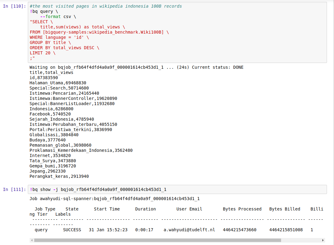
The dataset being aggregated is Wikipedia 100 billion records that have size ~ 4.5 TB. The script for the test is as follows.
#the most visited pages in wikipedia indonesia 100B records
bq query --format csv
"SELECT title,sum(views) as total_views FROM [bigquery-samples:wikipedia_benchmark.Wiki100B] WHERE language = 'id' GROUP BY title ORDER BY total_views DESC LIMIT 20;"
We aggregated 4.5 TB data and sorted the result. The result is remarkable! Only need 17 seconds to complete the operation.
Second test: end-to-end data processing (real-life scenario)
The first test seems to be idealistic, but in the real-life scenario, we have to take into account a number of things:
1) transport time, i.e., the time needed to transfer the data from our premises to Google Cloud Storage;
2) loading time, i.e., the time needed to load the data from Google Cloud Storage to Google BigQuery’s table
3) query time, i.e., the time needed to complete the query
For effective transport to the cloud, I compressed the data into gzip format. The data used in this test is the same data from the previous post (dataset). The findings are compared to the result of R data.table.
The following steps were being used:
1) Create a bucket in the nearest GCS to my location (I picked europe-west1: Belgium): gsutil mb -c regional -l europe-west1 gs://agungw132-dataset
2) Upload the file to the bucket using a parallel process: gsutil -m cp /scratch/awahyudi/d.csv.gz gs://agungw132-dataset
3) Create a dataset in GBQ repository (once more, EU is chosen to reduce the latency): bq mk -d --data_location=EU bigdata
4) Create a table in the dataset with the appropriate schema: bq mk -t bigdata.d x:string,y:float
5) Load the data from GCS to GBQ table: bq load bigdata.d gs://agungw132-dataset/d.csv.gz x:string,y:float
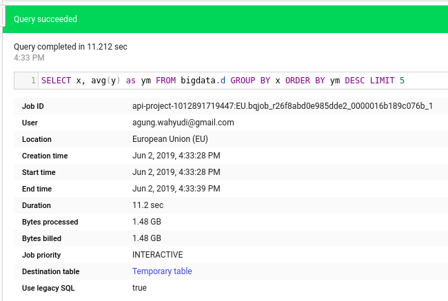
6) Aggregate and sort the data inside the table: bq query 'SELECT x, avg(y) as ym FROM bigdata.d GROUP BY x ORDER BY ym DESC LIMIT 5')
Then we put the entire commands into a single bash execution and measure the completion time.
time (gsutil mb -c regional -l europe-west1 gs://agungw132-dataset; gsutil -m cp /scratch/awahyudi/d.csv.gz gs://agungw132-dataset; bq mk -d --data_location=EU bigdata; bq mk -t bigdata.d x:string,y:float; bq load bigdata.d gs://agungw132-dataset/d.csv.gz x:string,y:float; bq query 'SELECT x, avg(y) as ym FROM bigdata.d GROUP BY x ORDER BY ym DESC LIMIT 5')
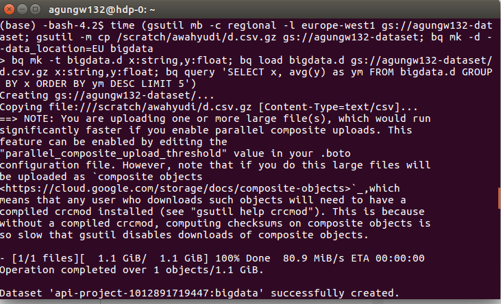
It took 5’3″ to complete the end-to-end data process.
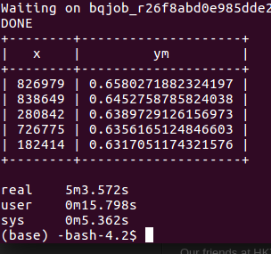
Checking from job history, it actually took only 11 seconds to complete the query time. It means that the transport and loading time spent the majority of elapsed time (~ 4’52”).
To investigate how much time which task spent the most time, I executed the following command.
time (gsutil mb -c regional -l europe-west1 gs://agungw132-public; gsutil -m cp /scratch/awahyudi/d.csv.gz gs://agungw132-public)
In a summary, breakdown of total completion time (5’3″) is transfer time from premises to GCS (33″), load data from GCS to GBQ’s table (4’19”), and query the aggregation & sorting (11″). The findings indicate that most of the time is spent in loading stage.
As a comparison, I used R data.table to perform the same operation (end-to-end data processing). The completion time is only 30 seconds!

Third test: comparing operation on GBQ’s table & external table
Google Big Query’s table (Baseline)
time (bq mk -t bigdata.d5 x:string,y:float; bq load bigdata.d3 gs://agungw132-public/d.csv.gz x:string,y:float; bq query 'SELECT x, avg(y) as ym FROM bigdata.d5 GROUP BY x ORDER BY ym DESC LIMIT 5')
Google Cloud Storage
time (bq mk --external_table_definition=x:string,y:float@CSV=gs://agungw132-public/d.csv.gz bigdata.d4; bq query 'SELECT x, avg(y) as ym FROM bigdata.d4 GROUP BY x ORDER BY ym DESC LIMIT 5')
Google Drive
$sw = [Diagnostics.Stopwatch]::StartNew(); bq mk --external_table_definition="x:string,y:float@C
SV=https://drive.google.com/open?id=183M8Am20cNutbs9UKKPL0R4dQyWPKb2L" bigdata.d12; bq query 'SELECT x, avg(y) as ym FRO
M bigdata.d12 GROUP BY x ORDER BY ym DESC LIMIT 5'; $sw.Stop(); $sw.Elapsed
As a summary, Google BigQuery has an amazing process time if the data is already in the GBQ tables. The transport time and loading time is so long that a single local R execution did a much better job than GBQ. However, if your data is too big to fit in RAMs and processing the data in a batch manner does not matter you (i.e., latency is not a concern), GBQ is suitable for you. Moreover, it suits you best if you do not want to buy any servers but need the job done.
1 thought on “Google BigQuery, a serverless Datawarehouse-as-a-Service to batch query huge datasets (Part 2)”