Next: Part 2

Google Big Query (GBQ) as a serverless service from Google
Serverless is one of big data solution to watch in 2018 according to Computer World UK (/compwuk). Google BigQuery (GBQ) is an example of enterprise-grade serverless service (either Function-as-a-Service, FaaS or Datawarehouse-as-a-Service) offered by Google Cloud Platform.
GBQ was first launched as a service in 2010 with general availability in November 2011. It is perfectly used to query such a massive dataset (petabyte-scale) in a batch manner and get the result very quickly. Can you imagine such a scenario that requires you to delve in a huge dataset, e.g.:
- A director suddenly asks, “Can you give me this month’s cumulative traffic, but only in the Jakarta region?”.
- After getting the number, he then continues, “Show me the month-on-month and year-on-year comparison both single month and cumulative!”
- And tons of other follow-up questions are the rest of the story.
The above scenarios are inevitable in real-life business, especially in the very dynamic business environment. For years, data analysts are looking ways to answer those questions. However, the technology, i.e., data warehouse, that was addressing those questions could not catch up the rate of questions asked by data consumers. Very often, data consumers have to wait for the questions to be answered in days even months; at the time on which the question is not timely relevant anymore.
In their white paper, Google claims the blazing performance of GBQ over traditional datawarehouse, i.e., executing a complex regular expression text matching on a huge logging table that consists of about 35 billion rows and 20 TB is completed in merely tens of seconds (/googlewp).
Also, GQP now integrates with varied services of Google Cloud Platform (GCP) and third-party tools which makes it easier to integrate and more applicable in many business cases.
How much should we pay for this technology? Since it is a serverless service, there is no infrastructure cost that we should pay. The schema for the cost is pay-as-you-use (PAYU) without any commitment fee. The cost includes a number of fee types, i.e.,
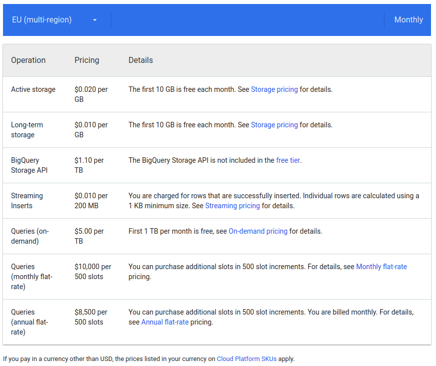
- Storage cost, i.e., the cost for saving data/query result to GBQ table permanently. It ranges from $0.01-0.02/GB (First 10 GB is free each month). As an illustration for 1 TB GBQ table, we have to pay $10 for long-term storage and $20 for active storage every month. A stored table that has not been updated more than 90 consecutive days is categorized as “long term”; otherwise it is active storage.
- Query cost, i.e., the cost of having GBQ performs data processing. We can select whether to use on-demand or bulk pricing scheme. On-demand query costs $5/TB (First 1 TB is free), meanwhile the bulk scheme costs $10K per 500 slots per month (monthly subscription) or $8.5K per 500 slots per month (annual subscription) regardless how huge data you process.
- Streaming insert cost, i.e., the cost of having GBQ loads streamed data (such as from its SaaS like PubSub) to GBQ table in real-time fashioned. For 200 MB data, we have to pay $1.1. The billing counts per inserted rows. The smallest billing unit for each row is 1 KB.
- GBQ Storage API cost, i.e., the cost of using GBQ storage API for ingesting GBQ table in a streamed manner to the client. For streaming 1 TB data via GBQ Storage API, GBQ costs $1.1.
This following article (/gcqcost and /gcqcost2) discusses how to calculate GCQ cost in detail.
GBQ architecture
Investigating GBQ architecture is useful to better how GBQ allocates resources so that query performance and storage optimization could be achieved.
GBQ is inspired by Google’s Dremel technology which has been internally used in production since 2006. Original Dremel papers were published in 2010 and at the time of publication, Google was running Dremel instances ranging from tens to thousands of nodes. Dremel is originally used as the interactive ad-hoc query system for analysis of read-only nested data. It incorporates columnar storage and tree architecture for processing huge data.
However, GBQ is wider than Dremel which is just an execution engine for the BigQuery. In fact, GBQ combines Dremmel with other Google’s innovative technologies such as Borg, Colossus, Capacitor, and Jupiter.
As explained by panoply.io (/bqarch2), a GBQ client (either web UI, bg command-line tool, or REST APIs) sends a job (i.e., query data and store the result) to Dremel engine via a client interface. Amount of computing required by Dremel to complete the job is managed by Borg – Google’s large-scale cluster management system. Dremel communicates with Google’s Colossus file systems via Jupiter network to read or write GBQ’s tables relevant to the job. Jupiter network enables GBQ-Dremel data transfer up to 1 Petabit/sec of total bisection bandwidth.

GBQ architecture decouples storage (Colossus), compute (Borg), and query engine (Dremel). By doing so, elasticity is easier to achieve, i.e., by scaling out/down the relevant entity. This elasticity capability makes GBQ more powerful than other datawarehouses.
Storage
GBQ stores each field (or column) of a data in columnar format, namely Capacitor, in separate files. By doing so, very high compression ratio and scan throughput can be obtained. Capacitor, released in 2016, is the replacement of ColumnIO, the former generation optimized columnar storage format. Capacitor allows GBQ to directly ingest a compressed data, without decompressing it first and processing the data on the fly. Before loading the data to Collossus (i.e., GBQ’s table), GBQ encoded every column separately into multiple Capacitor-formated files.
Colossus, Google’s latest generation distributed file system, replaces GFS (Google File Systems). Colossus handles cluster-wide replication, recovery and distributed management. It also implements a sharding strategy evolving based on the query and access patterns. The highest availability is achieved by having geo-replication of data across different data centers.
As a summary, Colossus allows splitting of the data into multiple partitions to enable blazing fast parallel read whereas Capacitor reduces requires scan throughput. Together they make possible to process a terabyte data per second.
GBQ is also capable to perform queries against external data sources (Google Cloud Bigtable, Google Cloud Storage, and Google Drive) without the need to import data into Colossus. When using this external data source, GBQ performs on-the-fly loading of data into Dremel engine. Usually processing external data sources will be slower than from Colossus. If performance is a concern, always import the data into GBQ’s table (i.e., Colossus) before doing any table operation (i.e., SQL queries).
Compute
GBQ utilizes Borg for spinning up simultaneously runs thousands of Dremel jobs across one or more clusters made up of tens of thousands of machines. Moreover, Borg also handles fault-tolerance.
Query Engine
Dremel engine uses a multi-level serving tree for scaling out SQL queries that are specifically designed to run on commodity hardware. A query dispatcher is used to not only provide fault tolerance but also schedule queries based on priorities and the load.
In a serving tree, a root server receives incoming queries from clients and routes the queries to the next level. To parallelize the query, each serving level (i.e., root and mixers) performs query rewrite and ultimately modified and partitioned queries reach the leaf nodes for execution. The query is modified to include horizontal partitions of the table, i.e., shards (in original Dremel paper shards were referred to as tablets). Leaf nodes of the serving tree do the heavy lifting of reading the data from Colossus and performing filters and partial aggregation. Each leaf node provides execution thread or number of processing units often called as slots. It is important to note, Dremel automatically calculates how many slots should be assigned to each query. The number of allocated slots depending on query size and complexity. At the time of writing of this article, for on-demand pricing model maximum 2000 concurrent slots are allowed per BigQuery project. Leaf nodes return results to mixers or intermediate nodes. Mixers perform aggregation of results returned by leaf nodes.
The following scenario illustrates the process in Dremel.
Supposed a client sent a query (i.e., aggregation column B grouped by column A from table T) to root server:
SELECT A, COUNT(B) FROM T GROUP BY A
Root server translates the query into a simplified form that represents determines all shards of table T and sends it to mixers. In this case, R11, R12,..., R1n are results of queries sent to the Mixer 1, . . . , n at level 1 of the serving tree.
SELECT A, SUM(c) FROM (R1i UNION ALL ... R1n ) GROUP BY A
Leaf nodes receive the queries and read data from Colossus shards. A Lead node reads data for columns or fields mentioned in the query. As leaf node scans the shards, it walks through the opened column files in parallel, one row at a time. For example, mixer 12 translates R12 shard to R22 and R23 and send it to leaf node 22 and 23.
Optimization based on the architecture
Depending on the queries, data may be shuffled between leaf nodes. For instance, for GROUP EACH BY in queries, Dremel engine will perform shuffle operation. It is important to understand the amount of shuffling required by your queries. Some query with operations like JOIN can run slow unless you optimize them to reduce the shuffling. That’s why GBQ recommends trimming the data (i.e., removing or excluding unnecessary rows) as early in the query as possible so that shuffling due to your operations is applied to a limited data set.
As BigQuery charges you for every 1 TB of data scanned by leaf nodes, we should scan based on our need, not too much or too frequent. There are many ways to do this.
- One is partitioning your tables by date. For each table, additional sharding of data performed by GBQ which you can’t influence.
- Instead of using one big query, break them into small steps and for each step save query results into intermediate tables so that subsequent queries have less data scan.
- It may sound counter-intuitive but the LIMIT clause does not reduce the amount of data get scanned by a query. If you just need sample data for exploration, you should use Preview options and not a query with the LIMIT clause.
At each level of serving tree, various optimizations are applied so that nodes can return results as soon as they ready to be served. This includes tricks like priority queue or streaming results.
GBQ and its competitors
GBQ has strong competition from other cloud providers, such as Amazon Redshift (/redshift) from AWS and SQL Datawarehouse (/azuresql) from Azure.
Comparing the performance
Next: Part 2